Digital Twins & AI

From Concept to Reality

Building Intelligent Environments for a Sustainable Future

Type this URL into your browser:

bit.ly/ie26tut4

Introduction

Myself: Gian Marco Paldino

Postdoctoral Researcher · Machine Learning Group, ULB · Ph.D. 2026

Research focus: multivariate time series — causal inference, forecasting, anomaly detection, and Digital Twins.

Today:

MLG-ULB — What We Do

Founded in 2004 by Prof. Gianluca Bontempi, is currently co-headed by him and Prof. Tom Lenaerts. MLG targets machine learning and behavioral intelligence research on time series analysis, big data mining, causal inference, network inference, decision-making models and behavioral analysis

The EDITS project (Enhancing DIgital TwinS with scalable and interpretable AI) — funded by WEL-T

Energy Twin / VPP — Energy Communities, distributed energy management

Traffic Twin — Urban roadwork impact, Traffic Simulation

Human / Robotics Twin — EMG fatigue modelling, musculoskeletal rehabilitation

Causal AI — Transfer learning across assets, what-if & counterfactual reasoning

The EDITS Project & WEL-T

EDITS: Enhancing Digital Twins with Scalable & Interpretable AI.
Made possible by funding from WEL-T.
Our Goal: Move Digital Twins from academic buzzwords to deployed, AI-driven solutions in Energy, Mobility, and Manufacturing.

Agenda (2 Hours)

14:00 - 14:20	Theory: The Digital Twin Architecture
14:20 - 14:50	Hands-on 1: The Physical Twin (Data Generation)
14:50 - 15:00	10 minutes break
15:00 - 15:20	Hands-on 2: The Digital Brain (Machine Learning)
15:20 - 16:00	Hands-on 3: Closing the Loop (Optimization)

Assumptions: basic Python / basic ML knowledge. Google colab, internet.

Digital Twins

A CAD model.

Is this a Digital Twin?

NO This is a Digital Model

A movie made from real life sensors.

Is this a Digital Twin?

NO This is a Digital Shadow

A robotic hand moving in real-time.

Is this a Digital Twin?

YES Digital and physical inform each other continuously

What is a Digital Twin?

Not just a static 3D model.
Sensing: Data updates the virtual model.
Actuating: DT affects real-world decisions.
Digital Shadow: green arrow only. (e.g.
Digital Model: orange arrow only. (e.g. CAD tools)

The 5-Layer Architecture

Generation: Sensors, IoT, Simulators
Streaming: Kafka / Big Data
Storage: Time-Series Databases
Processing: Machine Learning & AI
Decision: Dashboards & Optimization

Virtual Power Plants

Today's Use Case: The Virtual Power Plant

A Virtual Power Plant (VPP) is a cloud-based distributed power plant that aggregates the capacities of heterogeneous distributed energy resources (DERs) — solar panels, wind turbines, battery storage, and flexible loads — and coordinates them as a single, dispatchable unit visible to the grid operator.

No single physical location — exists as software + communication layer.
Compensates for the intermittency of renewables by pooling complementary assets.
Key metric: keep supply = demand at all times (grid frequency = 50 Hz).

VPP — Under the Hood

Components

☀️ Solar PV panels
💨 Wind turbines
🔋 Battery storage (BESS)
🏭 Flexible industrial loads
🏠 Smart-meter households

What the DT does

Forecasting: predict solar & wind output (LSTM, XGBoost)
Scheduling: charge/discharge battery optimally (LP/MPC)
Market participation: bid surplus into day-ahead markets
Fault detection: anomaly detection on sensor streams

Why VPP is a Textbook Digital Twin

Sensing (Physical → Digital)

Solar irradiance & wind speed → update forecast model
Battery state-of-charge → update optimisation state
Household consumption → update demand model

Actuating (Digital → Physical)

Optimised schedule → commands inverters & BESS
Market bid → triggers real energy transactions
Fault alert → triggers maintenance crew

Both arrows active → true Digital Twin,
not just a shadow or a model.

VPP — Real-World Deployments

Next Kraftwerke (Germany) — Europe's largest VPP, >14 GW aggregated capacity from 13 000+ assets. Trades energy on 9 European spot markets in real-time.

Tesla Autobidder (Australia) — Hornsdale Power Reserve (150 MW / 194 MWh BESS). Automated battery dispatch saved the Australian grid ~$150 M AUD in frequency regulation costs (2018–2020).

Ørsted / Danish TSO — Offshore wind VPP that curtails or ramps turbines within seconds to balance the national grid; integrates weather-forecast ML models updated every 15 min.

Hands-on 01 - Data generation

In simple terms

We get weather data and use specialized libraries that convert this weather data into energy profiles for solar panels and wind turbines.

🌐 Weather Data Input

Temperature, irradiance, wind speed, humidity, cloud cover, etc. from weather stations or forecasts.

⚙️ Specialized Libraries

pvlib (solar), windpowerlib (wind), and others that model physics & efficiency.

⚡ Energy Profile Output

Predicted power output (kW/MW) for each asset at each time step—ready for optimization.

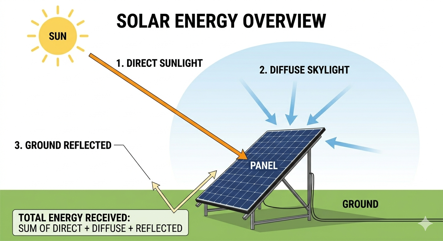
Solar Irradiance

Solar Irradiance

The sun's energy reaching a surface splits into three components that pvlib needs separately.

☀️ GHI — Global Horizontal Irradiance

Total solar radiation on a flat horizontal surface. GHI = DNI·cos(θ) + DHI. The "headline" number from weather stations.

🔆 DNI — Direct Normal Irradiance

Radiation arriving directly from the sun's disk, measured on a surface always perpendicular to it. Dominant on clear days. Strongly affected by tilt & azimuth.

🌫️ DHI — Diffuse Horizontal Irradiance

Scattered radiation from the rest of the sky dome (clouds, atmosphere). Does not depend on panel orientation — you always receive it.

Why all three? A tilted panel sees a different mix of direct, diffuse, and ground-reflected light. pvlib needs all three to compute what actually hits your panel.

How pvlib Works — The Model Chain

pvlib strings together a pipeline of physical models. Each step converts one quantity into the next:

1. Solar position → sun altitude & azimuth from lat/lon/time (ephemeris)

2. Plane-of-Array (POA) irradiance → project GHI/DNI/DHI onto your tilted surface using the angle of incidence (AOI)

3. Cell temperature → Faiman / Sandia thermal model; higher temp = lower power

4. DC power → PVWatts or SDM model using POA & cell temp

5. AC power → inverter efficiency curve (SNEC / PVWatts)

The columns ghi, dni, dhi, temp_air, wind_speed are the exact inputs steps 1–3 consume — that's why the names are mandatory.

PV System Parameters — Physical Meaning

Module

pdc0 = 250 W — rated DC power at Standard Test Conditions (1000 W/m², 25 °C). The nameplate figure on the panel datasheet.

gamma_pdc = −0.0045 — temperature coefficient (%/°C). At 60 °C (typical summer) power drops by ≈ 0.45 % × 35 °C ≈ −16 %. Negative because silicon efficiency falls with heat.

surface_tilt = 30° — angle from horizontal. Closer to your latitude → more annual energy; steeper → better winter, worse summer.

surface_azimuth = 180° — South-facing (Northern Hemisphere). Maximises daily sun exposure. 90° = East, 270° = West.

Inverter & Racking

pdc0 = 240 W — inverter DC input limit. Slightly below panel rating → clips only rare peak moments, optimises cost.

eta_inv_nom = 0.96 — 96 % conversion efficiency DC→AC. Losses are heat in the electronics.

open_rack — panels mounted with air flowing behind them; cooler → better efficiency. "close_mount" (roof-flush) runs hotter.

glass_polymer — back-sheet material; affects thermal model coefficients (emissivity, absorption).

Wind Power

Wind power follows a cubic law — small speed changes have a huge impact.

Key physics

P ∝ v³ — doubling wind speed → 8× more power. Above rated speed, the turbine pitches blades to cap output.

Cut-in speed (~3 m/s) — minimum wind to start generating. Below this: 0 W.

Rated speed (~12 m/s) — turbine reaches nameplate power; output plateaus.

Cut-out speed (~25 m/s) — turbine shuts down to avoid structural damage.

What we model

wind_speed column — measured at 10 m height (standard met station). We scale to hub height (~80 m) with a log-law profile.

Power curve — manufacturer's lookup table mapping v → P. We interpolate it in the notebook.

Capacity factor — actual energy ÷ theoretical max. Typical onshore: 25–35 %. Offshore: 40–50 %.

3. Simulating Community Demand & Tariffs

Build a realistic load profile and dynamic price signal for downstream prediction.

Demand profile

Base demand — lower weekends (5 kW) and weekdays (7 kW).

Morning peak — Gaussian bump around 08:30 with a smaller amplitude than the original model.

Evening peak — wider peak around 19:30 to capture after-work usage.

Noise + floor — adds small hourly variation and clips demand to a 2 kW minimum.

Dynamic tariff

Base price — starts at €0.15/kWh.

Peak premium — adds cost during morning and evening demand windows.

Solar damping — reduces price when local solar generation is high, echoing the duck curve.

Volatility — small random variation keeps the price signal more realistic.

Clipping — keeps tariffs within a practical range.

Hands-on 02 - Training the Digital Brain 🧠

Predictive Modeling for the Digital Twin

Supported by the WEL Research Institute (WEL-T) - EDITS Project

1. Embedding: Time Series to Tabular

Standard ML models require independent rows to predict a target.

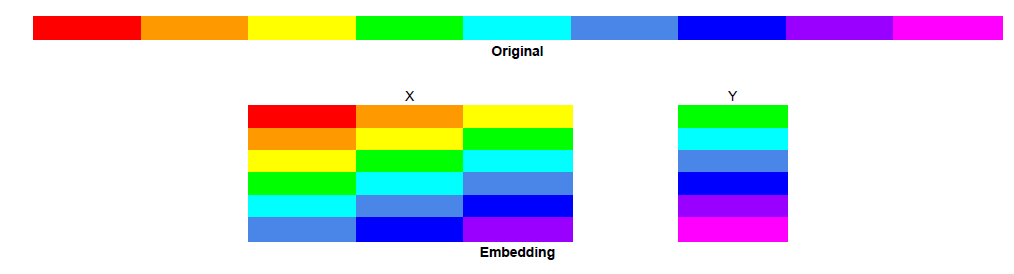
Lag Embedding: We reconstruct the phase space of the time series by mapping a single continuous signal into a multi-dimensional row vector using past values:

The maxlags Parameter (d)

Defines the lookback horizon of the model.
Must balance historical context with data loss (each lag introduces NaNs at the beginning of the series).

Leakage Prevention

Lags must only look backward (using positive shifts like shift(1)).
Any forward shift (e.g., shift(-1)) introduces future data into the current training row.

2. Feature Extraction

Condensing historical windows into compact statistical summaries.

Why extract statistical features? Relying solely on individual lags to capture long-term context leads to high-dimensional, highly correlated feature matrices. Rolling statistics summarize the properties of a window without adding excessive columns.

Rolling Operators

Rolling Mean: Captures the local smoothed trend level.
Rolling Std: Quantifies recent volatility (useful for highly variable sources like wind).
Rolling Min/Max: Captures recent local boundaries.

Causal Constraints

Rolling operations must be right-aligned (using center=False).
Centered windows look forward in time, violating temporal boundaries and causing severe validation leakage.

3. Feature Engineering

Injecting domain-specific physical and temporal structures into the model.

Cyclical Signal Encoding

Linear features like Hour (0–23) hide temporal proximity (hour 23 and hour 0 are close, but numerically far). We map these inputs to a 2D coordinate space using sine and cosine transformations:


                        Hour_Sin = sin(2π·h/24), Hour_Cos = cos(2π·h/24)

Mitigating Dimension Explosion

Adding lags and rolling windows to every exogenous signal causes feature count to balloon quickly. We selectively include current physical drivers (like Global Horizontal Irradiance, ghi) without lagging them, keeping the feature space compact.

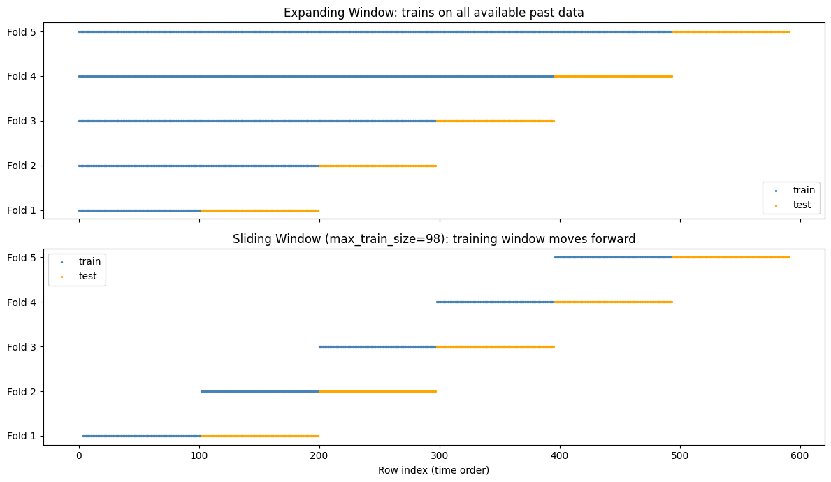
4. Time Series Cross-Validation (TSCV)

Evaluating models without violating the direction of time.

5. Normalized Mean Squared Error (NMSE)

Evaluating predictive skill relative to trivial averages.

Raw Mean Squared Error (MSE) is highly scale-dependent, making it difficult to compare performance across different physical locations, scales, or variables.

The Formula


                        NMSE = MSE / Var(y_true)

Normalizing by the variance of the target ground truth converts the error into a relative, scale-independent metric.

Interpretation Rules

NMSE > 1: The model performs worse than a simple historical mean forecast.
NMSE ≈ 0: Near perfect alignment with reality.
Equivalence: 1 - NMSE represents the Coefficient of Determination ($R^2$).

6. Scaling Up & Recursive Forecasting

Extending predictions across multiple variables and long-term planning horizons.

System-wide Scaling: To build a functional Digital Twin, we replicate this tabular workflow for all key dynamic variables (including load demand, wind generation, and thermal variations).

Recursive Forecasting Concept

Standard models predict only one step ahead ($t+1$). For multi-step horizons (e.g., $t+24$ for battery scheduling), we feed the predicted value at $t+1$ back into the lag array to predict $t+2$, iterating step-by-step.

Error Propagation Challenge

Because recursive forecasting uses predicted values as inputs for subsequent timesteps, any error introduced early in the chain propagates and compounds as the forecast horizon expands.

Hands-on 03 - Optimization

Energy Arbitrage

The same principle as buying low and selling high — applied to electricity.

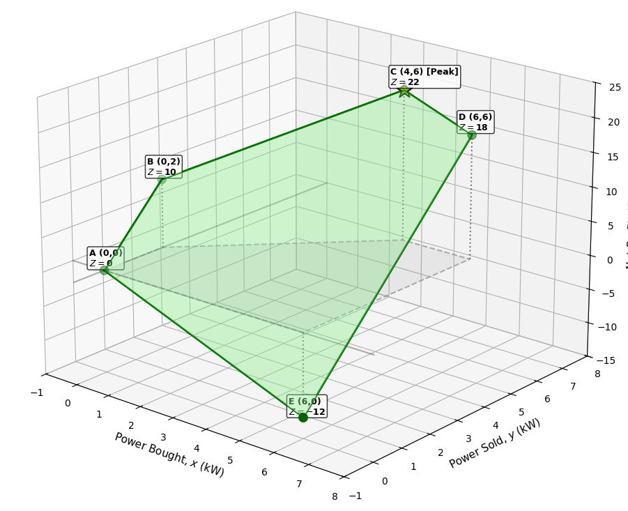
Why do prices fluctuate? Electricity cannot be stored at grid scale cheaply. When renewables overproduce (midday sun), supply > demand → prices crash. Evening peak → prices spike. Day-ahead markets (EPEX, Entsoe) clear hourly.

Arbitrage opportunity — charge a battery when cheap (night or solar surplus), discharge and sell when expensive (evening peak 17:00–21:00). Profit = revenue_sell − cost_charge.

Optimization: simplex idea

Setting up the search space before we visualize it

The Mathematical Setup

1. Decisions:
x = Power bought (Costs $2/kW)
y = Power sold (Earns $5/kW)

2. Objective:
Maximize profit Z = 5y - 2x

3. The Walls (Constraints):

Grid connection limit: x ≤ 6 and y ≤ 6
Physical battery capacity: y ≤ x + 2 (SOC)
No negative power: x ≥ 0, y ≥ 0

The Optimization Logic

These constraint lines intersect to form a 5-sided polygon on a 2D plane.

Key fact: because the objective is linear, the optimum always sits at a corner of this shape.

Simplex starts at one corner and hops to a better neighboring corner until convergence.

Visualizing the constraints

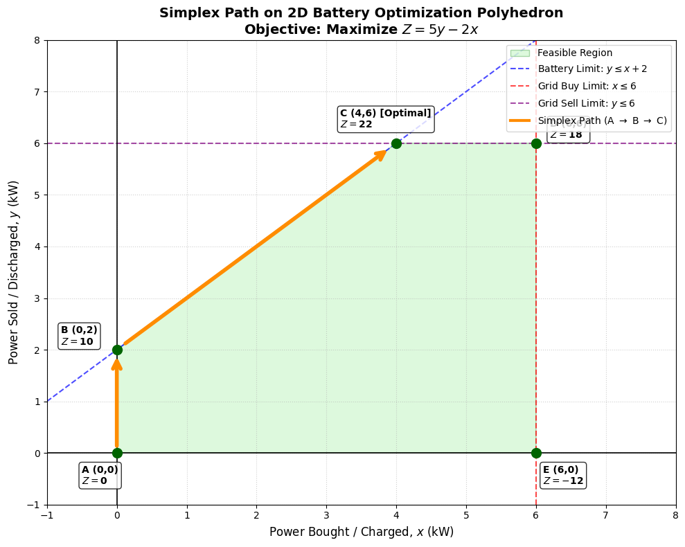
Feasible region polygon with vertices and optimal corner highlighted

Visualizing the profit

What is PuLP, really?

PuLP is a translator, not a solver. It lets you write optimization problems in readable Python (prob += ...), then translates them into a standard mathematical format.

It hands that off to an actual solver — by default CBC (COIN-OR Branch and Cut), bundled with PuLP.

prob.solve() calls CBC, waits for it to finish, and reads the result back into your Python variables via .varValue.

pulp.LpStatus[status] tells you what CBC reported: Optimal, Infeasible, or Unbounded.

Our case in Math

\[ \min \sum_{t \in T} \left( P_{\text{buy}, t} \cdot p_{\text{buy}, t} - P_{\text{sell}, t} \cdot p_{\text{sell}, t} \right) \]

→ This is the objective function. A sum of variables × constants — fully linear.

\[ PV_t + W_t + P_{\text{buy}, t} + P_{\text{discharge}, t} = D_t + P_{\text{sell}, t} + P_{\text{charge}, t} \quad \forall t \in T \]

→ Energy balance constraint. Repeated for every hour $ t \in T $.

\[ SoC_t = SoC_{t-1} + (P_{\text{charge}, t} \cdot \eta) - \frac{P_{\text{discharge}, t}}{\eta} \quad \forall t \in T \]

→ Battery dynamics constraint. Links hour $ t $ to hour $ t-1 $

Our case in Python

prob += pulp.lpSum([P_buy[t]*price_buy_f[t] - P_sell[t]*price_sell_f[t] for t in times])

→ This is the objective function. A sum of variables × constants — fully linear.

prob += (pv_f[t] + wind_f[t] + P_buy[t] + P_discharge[t] == demand_f[t] + P_sell[t] + P_charge[t])

→ Energy balance constraint. Repeated for every hour $ t \in T $.

prob += (SoC[t] == SoC[t-1] + (P_charge[t] * eta) - (P_discharge[t] / eta))

→ Battery dynamics constraint. Links hour $ t $ to hour $ t-1 $

Ok but... 24 hours?

PuLP doesn't solve hour by hour. It sees the whole 24-hour problem as one big system of equations.

The solver looks at the entire 24-hour horizon in a single mathematical step. It decides to charge the battery at 2:00 AM because it already sees the high prices at 2:00 PM and knows that is the globally optimal path to minimize total cost.

Where to go from here

Kafka to stream the data.

Time series database to store the data.

MLflow to handle the ML part.

Docker to package everything and deploy it to the cloud.

Thank you for your attention

For slides; code; and paper